
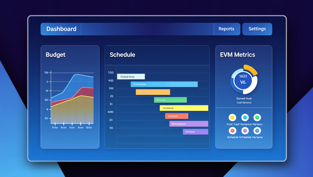
A plain-English guide to knowing whether your project is really on track
The Question Every Project Manager Dreads
“So… how’s the project going?”
Example Project
Excavate 200,000 m³ of material over three months, budgeted at $10 per m³, giving a total budget of $2,000,000.
In EVM the total budget has a formal name, the Budget at Completion (BAC). File that away; it becomes important when we forecast the final cost later.
The schedule is more than an end date. It directs how much work is meant to happen in each period. For our example, production ramps up while crews and equipment settle into the job, so month 1 plans less volume than the following months. To keep the example simple, all costs are carried in the single $10/m³ rate and establishment and overheads are ignored.
| Month | Planned volume | Planned spend | Cumulative planned spend |
| 1 | 60,000 m³ | $600,000 | $600,000 |
| 2 | 70,000 m³ | $700,000 | $1,300,000 |
| 3 | 70,000 m³ | $700,000 | $2,000,000 |
End of Month 1
Month 1 ends and the costs are in: you have spent $480,000 against a plan of $600,000.
Good news? You genuinely cannot say yet. Think about what that figure does and does not tell you:
- If the crews moved the full 60,000 m³ planned for month 1, you are a hero: all the month’s work for $120k less than budgeted.
- If they moved well short of that, you have an issue: most of the month’s money is gone, part of the month’s work is missing, and the remaining dirt will have to be moved with less budget than the plan allowed for it.
A pure cosr report cannot tell these two situations apart. Both show “$480k spent against a $600k plan”, and both would be reported as “$120k under budget”.
Then the survey data arrives: the crews moved 40,000 m³, two-thirds of the plan. It is the second situation. The information missing from the cost report is what the completed work was worth, and that is the “earned value” in Earned Value Management.
How Do You Actually Measure “Work Completed”?
Before work starts, each work package is assigned a Rule of Credit (RoC), a pre-agreed method for when value is earned, typically:
- Physical Units complete: for repetitive, countable work. The most objective method; use it wherever you can count something.
- Weighted milestones: for longer tasks with natural checkpoints. If our package included a dewatering pump station, it might earn 30% when set on its base, 40% when piped up, and 30% when commissioned.
- Percent complete: an assessed percentage, acceptable only with documented, verifiable criteria such as quantity surveys, because it is an easy method to game.
- Apportioned effort: for support work that shadows other work, like the survey crew checking the excavation. It earns value in proportion to the work it supports.
- 0/100: no credit until the task is finished. Best for short tasks; it removes all temptation to claim optimistic partial progress.
- Level of Effort (LOE): for ongoing overhead with no measurable output, like site management and security. LOE simply earns whatever was planned each period.
The Three Building Blocks: PV, EV, and AC
Every EVM calculation is built from three numbers, all expressed in hours, (or money), all measured at the same “status date”:
| Term | Also Known As | Meaning | Question It Answers |
| Planned Value (PV) | Budgeted Cost of Work Scheduled (BCWS) | What the work you planned to finish by now was budgeted to cost | “How much work should be done by now?” |
| Earned Value (EV) | Budgeted Cost of Work Performed (BCWP) | What the work you actually finished was budgeted to cost | “How much work was done?” |
| Actual Cost (AC) | Actual Cost of Work Performed (ACWP) | What you actually spent doing that work | “What did it really cost?” |
Earned Value (EV) is the last piece. Planned Value (PV) is $600,000 straight from our initial plan, and Actual Cost (AC) is $480,000 straight from the cost report. All we need now is the Earned Value, which identifies how much of the work was actually done against the plan. We work it out by taking the actual units moved and multiplying by the budgeted rate of $10/m³:
EV = 40,000 m³ × $10/m³ = $400,000
The project has banked $400,000 worth of progress regardless of what the ledger says it cost to achieve. That deliberate separation of budgeted worth from actual spend is what lets you compare “work done” against both the plan (PV) and the spend (AC).
CPI, the Cost Performance Index
We now know the project is over budget: $400k of work cost $480k. But raw dollar figures are hard to act on. Is an $80k overspend a disaster or a rounding error? It depends entirely on the size of the job. What a manager really needs is a measure of efficiency: how much work is each dollar buying?
That is exactly what the Cost Performance Index (CPI) provides. It divides the value of the work done (EV) by what was spent to do it (AC):
CPI = EV / AC
Because both numbers are in dollars, the result is a simple ratio centred on 1.0: below 1.0 each dollar is buying less than a dollar of work; above 1.0 it is buying more.
Our project: CPI = 400,000 / 480,000 = 0.83.
But how bad is 0.83? In theory 1.0 means exactly on budget, but in practice a perfect 1.0 is an anomaly; real work always carries some variance (LOE being the manufactured exception). So the index is typically read in bands:
| Band | Reading | Typical Response |
| 0.95 – 1.05 | Healthy. Normal noise around the plan | Keep monitoring |
| 0.90 – 0.95 | Underperforming. Needs looking into | Investigate cause, watch the trend |
| Below 0.90 | Serious trouble | Formal variance analysis and corrective action |
| 1.05 – 1.10 | Overperforming. Also needs looking into | Verify progress reporting and the baseline |
| Above 1.10 | A different kind of problem | Challenge the estimate and the data |
These bands are illustrative only. Every company (and often every contract) sets its own thresholds in its project controls procedures, and what one organization treats as “needs looking into” another may formally escalate.
The bottom two rows surprise people: how can doing too well be a problem? Because an index far above 1.0 rarely means heroic performance. More often the estimate was wrong or progress is being credited too generously. Even when it is genuine, it has commercial consequences: a client looking at CPI 1.25 doesn’t see a brilliant contractor, they see a padded price. High indices deserve the same scrutiny as low ones.
Our 0.83 sits well below the 0.90 line: not noise, not “needs watching”, but genuine trouble. Every dollar leaving the project is buying about 83 cents of excavation, which is the same fact as the $12/m³ actual unit cost expressed as a ratio. The ratio form matters because it is comparable across any package of any size: CPI 0.83 means the same thing on a $2M earthworks job or a $2B process plant.
SPI, the Schedule Performance Index
CPI answered the cost question, but our project has a second problem: less work has been done than the plan called for. Again, the raw gap ($400k done versus $600k planned) doesn’t immediately tell you how serious that is. What a manager needs is a measure of schedule performance: how much of the planned work has actually been accomplished by now?
That is what the Schedule Performance Index (SPI) provides. It divides the value of the work done (EV) by the value of the work the plan scheduled to be done by the status date (PV):
SPI = EV / PV
Our project: SPI = 400,000 / 600,000 = 0.67.
SPI is read against the same bands as CPI: 0.95 to 1.05 is healthy, below 0.90 is serious trouble, and far above 1.0 warrants the same scepticism about the baseline and the reporting. Our 0.67 says only two-thirds of the work that should be complete by now actually is: 40,000 m³ done when 60,000 m³ should be.
CPI vs. SPI Side by Side
Each index is useful on its own, but the sharper insight comes from reading them together. The pair pins down not just that the project is off plan, but what kind of problem it has:
- CPI > 1, SPI > 1: under budget and ahead. Genuinely excellent, or a padded baseline. Verify before celebrating.
- CPI > 1, SPI < 1: cost-efficient but slow. Classic sign of an under-resourced job: one excavator working productively when the plan assumed two.
- CPI < 1, SPI > 1: on pace but burning money. Typical of schedule-driven recovery: night shift, extra hired trucks, premium rates.
- CPI < 1, SPI < 1: over budget and behind. Corrective action needed.
In our project, both figures breach any reasonable threshold in the first month, so a formal variance analysis (root cause, impact on the final forecast, and a corrective action) is mandatory, not optional.
The Sibling Metrics: CV and SV
The same three building blocks also give you variances: the same story as the indices, expressed in dollars instead of ratios. Ratios are better for comparing packages of different sizes; dollar variances are better for explaining impact to a sponsor.
- Cost Variance: CV = EV − AC = 400,000 − 480,000 = −$80,000. We have spent $80k more than the completed dirt was worth.
- Schedule Variance: SV = EV − PV = 400,000 − 600,000 = −$200,000. We are $200k worth of excavation behind plan.
Forecasting the Future: EAC, VAC, and TCPI
The real payoff of CPI is that it lets you forecast where the project will land, not just describe where it is. This is where the BAC from Step 1 comes back.
Estimate at Completion (EAC): the forecast final cost, assuming current efficiency continues.
EAC = AC + (BAC − EV) / (CPI × SPI)
= 480,000 + (2,000,000 − 400,000) / (0.83 × 0.67)
= 480,000 + 1,600,000 / 0.56
≈ $3,360,000
What’s going on here? The money already spent ($480k) is sunk; the formula forecasts the remaining $1.6M of work at an efficiency dragged down by both the cost overrun and the schedule slippage. The result is sobering: a $2M package forecast to land at roughly $3.4M.
A simpler variant, EAC = BAC / CPI ≈ $2.4M, assumes only cost efficiency persists and the schedule problem costs nothing. The gap between the two forecasts, nearly $1M, is itself a message: on this project, the delay is expected to be as expensive as the digging.
Variance at Completion (VAC): the forecast overrun or underrun.
VAC = BAC − EAC = 2,000,000 − 3,360,000 = −$1,360,000
This is the overrun you should be warning the project manager about today, two months before it lands. Early warning is the entire point of EVM.
To-Complete Performance Index (TCPI): the efficiency needed on all remaining work to still finish on the original budget.
TCPI = (BAC − EV) / (BAC − AC) = 1,600,000 / 1,520,000 ≈ 1.05
To finish on $2M, the remaining 160,000 m³ must be moved at 5% better than budget, roughly $9.50/m³, by a team that has so far managed $12/m³. That is a big ask, and forcing that conversation is exactly what this number is for. When TCPI sits well above demonstrated CPI, the original budget is no longer credible: Fundamentally change how the work is being done, or look into change management.
A word of caution on forecasts. EAC, VAC, and TCPI are extrapolations, not predictions. They assume the future behaves like the past, and they know nothing about what is actually happening on the ground: the wet season ending, a renegotiated haulage contract, or a geotechnical surprise in the next cut. Treat the calculated figures as a starting point and a challenge to the team, never as the forecast itself. A credible EAC comes from combining the arithmetic with a bottom-up review of the remaining work, and where the two disagree, find out why before choosing which one to report.
Putting It Into Practice
- Build a solid baseline first. EVM measures against the plan, so a vague plan gives meaningless indices. You need a defined scope, a work breakdown structure, and a time-phased budget like our month-by-month table, with each chunk of work owned by one accountable person.
- Pick objective Rules of Credit per work package before work starts. Count things where you can (m³, metres, piles); minimize LOE.
- Measure on a regular cycle, monthly at minimum and weekly on fast-moving work, with agreed variance thresholds that trigger formal analysis.
- Watch trends, not snapshots. A CPI of 0.95 holding steady is a different animal from a CPI sliding 0.98 → 0.95 → 0.91 over three periods.
- Protect the baseline. Changes go through formal change control. Quietly re-planning to make the numbers look better destroys the meaning of every index.
- Report causes, not just numbers. “SPI is 0.67 because early rain delayed access to the main cut; recovery plan is a second truck fleet from week 6, EAC impact +$150k” is a report. “SPI is 0.67” is a complaint.
Limitations to Keep in Mind
- CPI and SPI describe past performance; they forecast well only when the future resembles the past.
- SPI ignores the critical path and converges to 1.0 at completion.
- Quality is invisible: you can earn full value on an excavated batter that fails geotechnical inspection next month.
- The outputs are only as honest as the baseline and the progress reporting feeding them.
Conclusion
Strip away the acronyms and EVM is three numbers and two divisions. What should be done (PV), what was done (EV), what it cost (AC); then CPI = EV/AC and SPI = EV/PV. On our earthworks package those two ratios turned a comforting “$120k under budget” cost report into the real story: a third of the planned work missing, and a forecast overrun of up to $1.4M arriving in two months unless someone acts. That is the whole promise of EVM: not more paperwork, but earlier warning signs.
The mechanics are simple, but making them work is not: building a credible baseline, choosing honest crediting rules, and turning the indices into decisions takes experienced project controls hands. If your project could use that kind of support, from setting up an EVM framework to running the reporting cycle, AUPY Consulting provides senior project controls personnel and PMO services for mining, EPC/M, and infrastructure operations. It is often a shorter conversation than a $1.4M variance meeting.